Seasonal Heat Pump Balance Point and Aux Heat Hours Calculator

Seasonal heat pump balance point introduction
This seasonal heat-pump balance point calculator estimates where a simplified building heating load matches the available compressor capacity. Below that modeled outdoor temperature, the table treats the difference between load and capacity as auxiliary-heat shortfall. It is intended for early retrofit planning: it helps show whether a proposed heat pump is likely to cover most of the heating load at the monthly temperatures and heating hours you enter.
Rather than selecting a preset climate, the model uses your building and weather assumptions. Envelope UA expresses whole-building heat loss in BTU/hr per °F of indoor-outdoor temperature difference. Continuous internal gains reduce the modeled load. The 47°F and 17°F capacity ratings establish a straight capacity line, which the calculator extends to each entered monthly average temperature. That makes the result useful for comparing a tighter envelope with stronger cold-weather equipment while keeping the same weather profile.
How to use the seasonal heat pump balance point calculator
- Enter the indoor heating setpoint and building UA. UA is the modeled whole-building heat-loss rate in BTU/hr·°F.
- Enter continuous internal gains and the heat pump's published heating capacities at 47°F and 17°F. The calculator uses these ratings to form its linear capacity curve.
- Review or replace each monthly average outdoor temperature and heating-hour estimate with values from your climate data, utility study, or project worksheet.
- Run the estimate and compare the balance point, modeled auxiliary hours, auxiliary energy, compressor coverage, and largest monthly shortfall. Use the CSV or copied summary when documenting alternate equipment or envelope assumptions.
Formulas behind the seasonal heat pump model
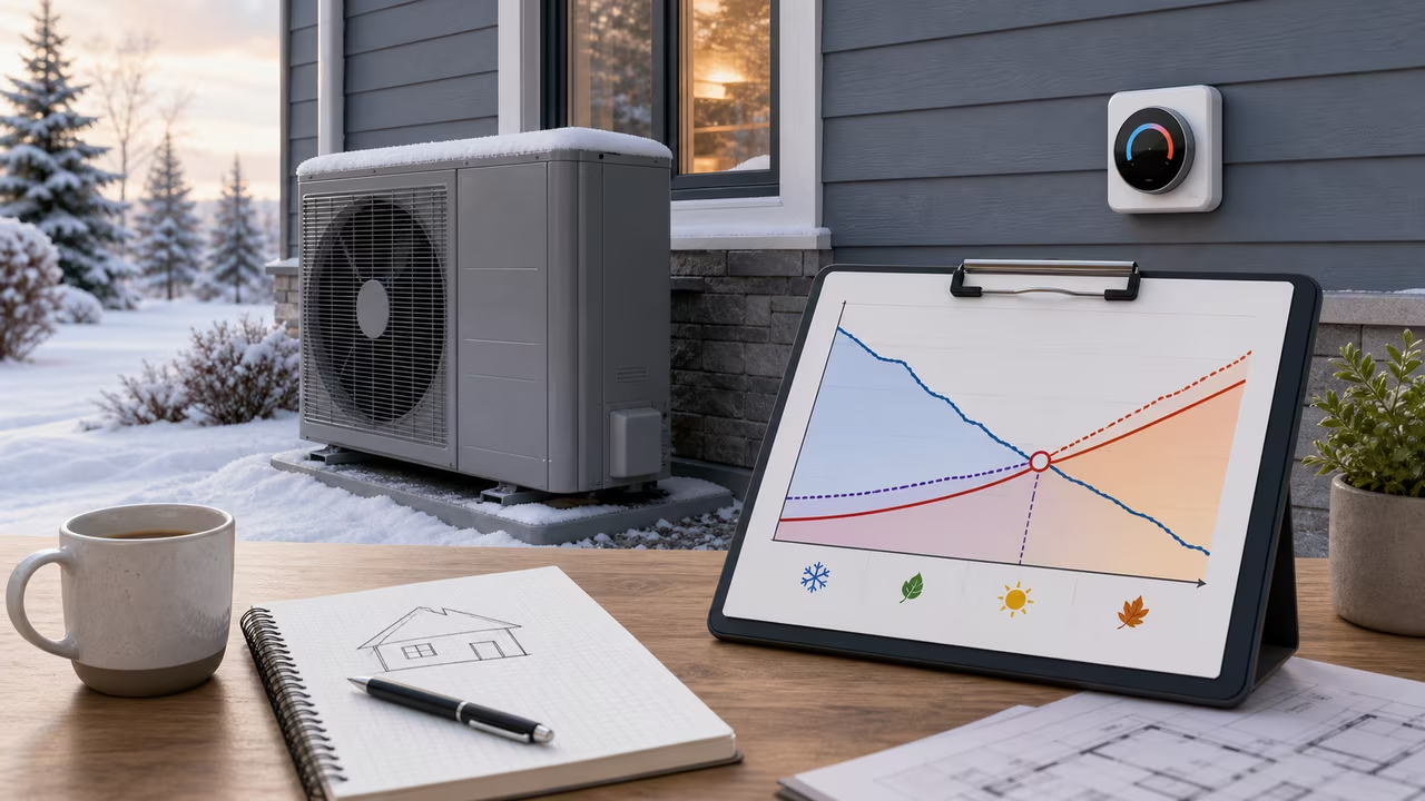
This heat-pump model compares a temperature-sensitive load with a temperature-sensitive capacity. As outdoor temperature falls, the UA-based load rises; the capacity line is determined by the two ratings you supply. Their intersection is the reported balance point. The model calculates building load as:
, where UA is the envelope heat-loss coefficient, is the indoor setpoint, is outdoor temperature, and is continuous internal gain. Negative loads are set to zero.
The available capacity is interpolated linearly from the 47°F and 17°F ratings. In formula form, the calculator uses . For a monthly bin, the shortfall is the positive part of load minus capacity. The displayed auxiliary share is that shortfall divided by load, and auxiliary hours equal this modeled share multiplied by the entered heating hours. Auxiliary energy is the shortfall rate multiplied by those heating hours.
Worked example: the calculator's default heat-pump assumptions
The default values provide a transparent check on the seasonal heat-pump calculation. They use a 70°F indoor setpoint, UA of 350 BTU/hr·°F, 3,000 BTU/hr of continuous gains, and capacities of 36,000 BTU/hr at 47°F and 22,000 BTU/hr at 17°F. Those ratings produce a capacity slope of about 467 BTU/hr per °F as outdoor temperature rises.
With those default building and equipment inputs, the two straight lines cross at about 9.1°F. The default monthly temperatures shown in the form are all warmer than that point, so the monthly-bin calculation shows no auxiliary shortfall for those averages. This does not mean a real installation can never call for backup heat: a monthly average can conceal colder hours, defrost behavior, duct losses, and thermostat staging. It does show why the weather bins and heating-hour values deserve the same scrutiny as the equipment ratings.
Comparing envelope and equipment strategies for auxiliary heat
Seasonal balance-point results are most useful when the same weather assumptions are run against several plausible envelope and equipment options. Lowering UA reduces the load at every outdoor temperature. Raising the 17°F rating relative to the 47°F rating improves the cold-side portion of the capacity line. The table identifies how each choice maps to an input in this particular model.
| Strategy | Modeled input effect | What to look for in results |
|---|---|---|
| Air sealing and insulation | Lowers UA, reducing the modeled load slope. | A lower balance point and less modeled auxiliary shortfall at the same temperatures. |
| Heat pump with stronger low-temperature output | Raises the 17°F capacity rating and changes the capacity slope. | More compressor coverage and a smaller shortfall in cold monthly bins. |
| Different backup staging controls | Does not change UA or the two capacity ratings entered here. | Not directly modeled; compare control behavior separately from this thermodynamic shortfall estimate. |
For each scenario, revise only the values that the proposal actually changes, then compare the resulting rows. A weatherization case should change UA, while an alternate heat pump should normally change one or both published capacities. The peak-shortfall result identifies the entered month with the largest rate gap; it is not a design load calculation or proof of required backup equipment size.
Interpreting seasonal heat pump coverage outputs
The seasonal heat-pump output separates modeled load served by the compressor from load assigned to auxiliary heat. Compressor coverage is an energy-weighted share: it divides modeled compressor-delivered load energy by total modeled load energy across all monthly bins. Auxiliary energy is reported in MMBTU from the same shortfall calculation, so it can be carried into a separate fuel-cost or electrical-service analysis if appropriate assumptions are added there.
The auxiliary-hours figure needs careful interpretation. It is not a record of literal resistance-strip runtime. The calculator converts each monthly load shortfall fraction into an equivalent share of the heating hours entered for that month. This is a compact way to compare scenarios consistently, but real controls may stage backup heat in shorter, more concentrated intervals or may run it for reasons not represented by the load-capacity comparison.
Use the balance point alongside the individual monthly rows. If it falls outside the range of entered monthly averages, the written interpretation explains what that means for this simplified profile. If a balance point lies within the entered range, inspect the adjacent cold-month rows rather than relying on the crossing temperature alone. The largest gap, total shortfall, and compressor coverage may each matter for different planning decisions.
Using the monthly heat-pump profile CSV
The seasonal heat-pump CSV download contains the same monthly profile displayed on the page: average temperature, modeled load, interpolated capacity, shortfall, auxiliary share, equivalent auxiliary hours, and auxiliary energy. It is useful for preserving the assumptions behind a scenario or comparing several equipment and UA combinations in a spreadsheet.
Keep the weather inputs consistent when comparing alternatives, and label exported files with the building and equipment assumptions used. A spreadsheet can then show which months drive the calculated shortfall and whether a lower-UA option or stronger low-temperature capacity changes the result more. The CSV remains a monthly-bin planning output, not measured operating data.
Seasonal heat pump balance point limitations and assumptions
This balance-point calculator intentionally simplifies heat-pump performance. Actual air-source capacity and efficiency do not necessarily follow a straight line between two ratings, and the code extends that line beyond the rating temperatures. Defrost cycles, airflow, duct performance, cycling, installation quality, and manufacturer operating limits can all change real delivered capacity. Monthly average temperatures also hide hour-to-hour weather swings.
The load model similarly treats UA and continuous internal gains as fixed. In practice, solar gain, wind-driven infiltration, occupancy, and thermostat schedules change over time. The model assumes the compressor supplies available capacity first and assigns any remaining modeled load to auxiliary heat. Use it to investigate direction and relative magnitude, then verify final equipment sizing, backup strategy, electrical requirements, and comfort expectations with detailed load calculations and manufacturer performance information.
| Month | Load (BTU/hr) | Capacity (BTU/hr) | Shortfall (BTU/hr) | Aux share of hours | Aux hours | Aux energy (MMBTU) |
|---|
Heat Pump Balance Point Freeze Run
Keep the compressor curve above the cold-weather load curve by collecting weatherization boosts and avoiding deep-freeze spikes. The game mirrors the calculator's main tradeoff: lower loads and stronger cold-weather capacity push auxiliary heat later into winter.
Balance capacity through cold snaps; green lowers load, amber boosts capacity, and blue adds cold stress.